Walking Zone Maps with Leaflet and Mapbox API

Your grandmother is elderly and hates driving. She is moving this year and has requested your assistance to help her find a new apartment in the city of Berkeley, CA. Since she cannot drive or walk very far, the apartment will need to be near a bus station for her to get around town and see friends.

Fortunately, the combination of R and the Mapbox API allow you to perform spatial analyses of walking and driving zones all over the world. Taking this analysis a step further, we can use a realty-listing API to map only 1-bedroom apartments within a short walk of local transit.

Load Packages

library(tidyverse)
library(leaflet)
library(mapboxapi)
library(sf)
library(httr)
library(jsonlite)

Find Local Bus Stations

The first step in the analysis of walking zones around bus stations is to find where the local bus stations are. There are a few options to accomplish this task. The most basic way to find the bus stations of a given geography is to check whether a nearby transit agency or government bureau offers transit data via an open data portal. Often, you will find there is a shp file with transit data that includes station names and location coordinates. (If you find only a csv file with latitude and longitude, make sure to find out which graphical coordinate system is used to project the data, else you may lead your grandmother astray.)

For this analysis, we will tap into the 511.org API, which provides transit data for the San Francisco Bay Area as well as other metropolitan regions. Since the purpose of this analysis is to look at walking zones, don’t sweat it if you find the next code chunk confusing. You can follow along with the main focus of the article.

To make our analysis more focused, we’re only going to look at the data for your grandmother’s most desired zip code in the city of Berkeley: 94705, an area just north of the lovely Bushrod Park.

# get key for 511 data from local R environment
key_511 <- Sys.getenv("KEY_511")

# format a httr request to get station data for AC Transit (short for Alameda County Transit)
resp <- GET("http://api.511.org/transit/stops",
            query = list(api_key = key_511,
                         operator_id = 'AC',
                         format = 'json'))

# extract json object using jsonlite package
# the :: feature lets you use a function from a package without calling library(package)
resp_json <- jsonlite::fromJSON(rawToChar(resp$content))

# shape data into tibble format
bus_station_sf <- resp_json$Contents$dataObjects$ScheduledStopPoint %>%
  as_tibble() %>%
  unnest_wider(Location) %>%
  select(id, Name, Longitude, Latitude) %>%
  st_as_sf(coords = c("Longitude", "Latitude"), crs = 4326)

# filter bus stations by Berkeley-Albany geography
options(tigris_use_cache = TRUE)
ashby_zip <- tigris::zctas(starts_with = c("94705")) %>%
  st_transform(crs = 4326)

berkeley_stops_sfc <- bus_station_sf %>%
  st_intersection(ashby_zip$geometry)

Generate Walking Zones

The fancy word for walking zones is “isochrones,” though if you say this word in a non-technical encounter you will surely confuse people. To generate isochrones, you can use the Mapbox API. Mapbox is GIS software that provides a variety of geospatial services, including custom map tiles and navigation APIs used by mobile apps like Uber and DoorDash.

Get your API Key

If this is your first time using the Mapbox API, you’ll need to obtain an API key from their website. To get an API key, create an account, head to the “tokens” tab, and follow the instructions to get your public API token. You can also create a secret token to read and write your own custom map data, though that will not be necessary for this analysis.

You can then store the key from your Mapbox API token in your R environment. This step is important since you never want to store your API keys in a script, especially when you may share or commit the script to version control.

# store your public api in your R environment
mb_access_token("your_public_api_key", install = TRUE)

Tip: To store any API key in your local R environment, you can open your environment using the code below. Add the key using the format YOUR_KEY_NAME = 'a_secret_api_key'.

Note that if you’re working on a collaborative project that requires regular sharing of API keys, you should consider using a managed service such as AWS Secrets Manager.

# this code will open a .Renviron script when run in RStudio
# add your api key to this script
file.edit("~/.Renviron")
# close this file when finished. Never check this file into version control

Request Geo-Spatial Data

Thanks to the work of GIS developer Kyle Walker, you don’t need to format an HTTP request or deal with a bulky software development kit to request walking zone data from the Mapbox API. Instead, we can use the mb_isochrone function in his R package ‘mapboxapi’. Using our simple features collection as the location argument, the function returns the walking zone around each location as a simple feature.

result <- mb_isochrone(location = berkeley_stops_sfc,
                       profile = "walking",
                       time = 2)

Map the Result with Leaflet

Now that we have all the areas in zip code 94705 that are located within a two-minute walk of a bus station, we can use the transport map provided by the Thunderforest API to provide us with further details about which bus line each stop is on. Now your grandmother has a better idea of where to look at apartments!

# merge overlapping polygons for a cleaner visual
result_unioned <- st_union(result)

# grab key for the use of Thunderforest API map tiles
# note that this is also a free service for small-scale, non-commercial use
key_thunder <- Sys.getenv('THUNDER_FOREST_KEY')
thunder_url <- 'https://{s}.tile.thunderforest.com/transport/{z}/{x}/{y}.png?apikey={apikey}'

# create a map using the leaflet package
my_map <- leaflet() %>%
  # alternatively you can simply call addTiles()
  addTiles(urlTemplate = thunder_url,
           attribution = 'Transit data © OpenStreetMap contributors',
           options = list(apikey = key_thunder)) %>%
  addPolygons(data = ashby_zip,
              fill = FALSE,
              color = 'blue',
              weight = 2) %>%
  addPolygons(data = result_unioned,
              color = 'green') %>%
  addCircleMarkers(data = berkeley_stops_sfc,
                   radius = .4,
                   # add hover-over label for different bus stops
                   label = ~Name)

my_map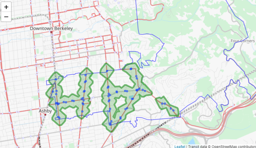

Leaflet map of South Berkeley showing the 94705 ZIP code in blue with green two-minute walking zones around bus stops

Add Apartment Listings

Realty Mole Property, a real estate technology company, offers an easy way to look at local real estate, home values, and other information important for renters and home buyers. You can tap into the API using the code below.

rapid_api_key <- Sys.getenv('RAPID_API_KEY')

url <- "https://realty-mole-property-api.p.rapidapi.com/rentalListings"

queryString <- list(
    city = "Berkeley",
    state = "CA",
    zipCode = "94705",
    bedrooms = "1",
    status = "Active",
    limit = "50"
)

response <- VERB("GET", url,
                 query = queryString,
                 add_headers('X-RapidAPI-Key' = rapid_api_key,
                             'X-RapidAPI-Host' = 'realty-mole-property-api.p.rapidapi.com'),
                 content_type("application/octet-stream"))

apt_listings <- fromJSON(content(response, "text")) %>%
  st_as_sf(coords = c("longitude", "latitude"), crs = 4326)

Using the sf::st_join() function, we can filter for apartments that are located within a two-minute walk of a bus station. Fortunately for your grandmother, this filtering option only eliminates a couple of options, so she has plenty of apartments left to choose from.

apt_listings_near_bus <- st_filter(apt_listings, result)

We can make a label for the filtered apartment listings and display them as markers on the map!

listing_label <- paste0(
  "Address: ", apt_listings$formattedAddress, '<br>',
  "Price: ", "$", apt_listings$price, '<br>',
  "Bedrooms: ", apt_listings$bedrooms, '<br>',
  "Property Type: ", apt_listings$propertyType) %>%
  lapply(htmltools::HTML)

my_map %>%
  addMarkers(
    data = apt_listings_near_bus,
    label = listing_label)

Going Further

In this article, we covered how to find local transit data and map the walking zone around transit stations. The framework established with the scripts above will easily allow you to apply this methodology to other regions and to analyze other types of isochrones. In addition to walking zones, you can use the Mapbox API to generate driving zones and the zones within a specified distance to a point of interest (e.g. a half-mile radius around the best ice cream shops).

Note that if you already have your geo-spatial data ready to go, you should consider using a platform like ArcGIS (paid) or QGIS (free) to perform this type of analysis. These platforms allow you to perform analyses of walking zones using little to no code. The only downside is that it can often be clunky to find your data online, download it, load it to one of the software platforms, and export the results. Performing these types of spatial analyses in R scripts has the key benefit of streamlining your GIS workflow.