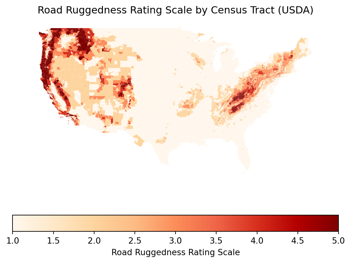
The U.S. government has released an unprecedented number of datasets in recent years. But these data are often released without accompanying geospatial data. Fortunately, Python libraries like Geopandas and Pygris make it easy to locate the geo data you need to perform your analysis.
For example, the USDA recently released a dataset detailing the ruggedness of roads by Census tract. The data could provide interesting insights for car companies, logistics firms, and others, but we need to map it first.
Load Libraries and Data
To accomplish this task, we’ll need to load a few libraries.
import pandas as pd
import geopandas as gpd
import numpy as np
from pygris import tracts
We can load the USDA data directly from the agency’s website using Pandas.
tract_ratings = pd.read_excel('https://www.ers.usda.gov/webdocs/DataFiles/107356/RuggednessScale2010tracts.xlsx?v=486.9')Since the USDA data is at the Census tract level, we’ll use Pygris to load the Census tract data.
The Python library Pygris was developed to make it easy to load Census tract data. The library contains a function called tracts that allows you to load Census tract data by state and county. Due to the configuration of the Census tract data, you’ll need to load the data by state.
Before running this code, make sure you have a strong internet connection. You will be downloading a large amount of data so be prepared to wait.
# Load list of states
states = pd.read_csv('https://raw.githubusercontent.com/jasonong/List-of-US-States/master/states.csv')

# Create list to store tract data
tract_list = []

# Fetch Census Tract Data using pygris
for abbreviation in states['Abbreviation']:
    print(abbreviation)
    state_tracts = tracts(year=2010, cb=True, cache=True, state=abbreviation)
    tract_list.append(state_tracts)

# geoDataFrame of all tracts
all_tracts = pd.concat(tract_list)
Merge Data
Now that we have both the USDA data and the Census tract data, we can merge the two datasets and extract the relevant columns.
# take string of GEO_ID following US and convert to int for merging
all_tracts['TractFIPS'] = all_tracts['GEO_ID'].str[9:].astype(np.int64)

# Merge tract info with ratings
merged_data = all_tracts.merge(tract_ratings, on='TractFIPS', how='inner')

# Filter columns
filtered_data = merged_data[['TractName', 'CountyName', 'State', 'Population', 'RRS', 'RRSDescription', 'geometry']]
Map Data Using GeoPandas
Now that we have the data we need, we can map it using GeoPandas.
Removing Hawaii and Alaska will simplify this task. If we did want to include these states in the map, we would want to extract their polygons and add them as insets below the mainland U.S. (Note that the tidycensus package of R lets you do this automatically).
# filter out Alaska and Hawaii
mainland_data = filtered_data[~filtered_data['State'].isin(['AK', 'HI'])]
With our data ready to go, we can finally map it in geopandas.
# Plot choropleth map with RRS as color
ax = mainland_data.plot(column='RRS',
        cmap='OrRd',
        legend=True,
        legend_kwds={'label': "Road Ruggedness Rating Scale", 'orientation': "horizontal"})

# Add title
ax.set_title('Road Ruggedness Rating Scale by Census Tract (USDA)')

# Remove axes from map
ax.set_axis_off()